Python3 Programming

●Hello, NumPy!!

• NumPy は数値計算を効率的に行うための拡張モジュール
• 多次元配列のサポートとそれを操作するための高度な数学関数が提供される
• 本ページでは基本的な使い方を簡単に説明する
• インストールは pip を使うと簡単

python3 -m pip install numpy

$ python3 -V
Python 3.10.6

$ python3 -m pip freeze | grep numpy
numpy==1.24.1

• numpy ver 1.24.1 がインストールされる (2023 年 5 月時点)
• 実行環境 : Ubunts 22.04 LTS (WSL2, Windows 10), Intel Core i5-6200U 2.30GHz
• pip は Python で書かれたパッケージ管理ツール
• 最新の Python は pip を同梱している
• あとは numpy をインポートするだけ

import numpy as np

• as を使うとモジュールに別名を付けることができる
• 下記の参考 URL を読むと、別名に np を付けるのが一般的なようである
• 参考 URL
• NumPy, (本家, http://www.numpy.org/)
• Numpy and Scipy Documentation, (本家, https://docs.scipy.org/doc/)
• Pythonの数値計算ライブラリ NumPy入門, (rest term さん)
• Numpy入門 - Python学習講座, (Kuro さん)
• python/numpy, (朱鷺の杜Wiki さん)

• 計算結果を画像で表示したい場合は matplotlib を使うとよい
• 次のコマンドで必要なパッケージをすべてインストールできる

python3 -m pip install matplotlib

$ python3 -m pip freeze | grep matplotlib
matplotlib==3.6.2

• 本ページでは matplotlib の説明は割愛する
• 基本的な使い方は下記参考 URL を参照
• 参考 URL
• Matplotlib, (本家, https://matplotlib.org/)
• User's Guide, (本家, https://matplotlib.org/stable/users/index.html)
• matplotlib 入門, (柞刈湯葉さん)
• matplotlib入門 - りんごがでている, (bicycle1885 さん)

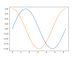
リスト : numpy と matplotlib の簡単な使用例

import math
import numpy as np
import matplotlib.pyplot as plt

x = np.linspace(0, 2 * np.pi, 100)
plt.plot(x, np.sin(x))
plt.plot(x, np.cos(x))

# plt.savefig("testplt.png", dpi=50)
plt.show()

●配列 ndarray

• NumPy の多次元配列は ndarray というクラス
• 固定長配列
• 要素は同じデータ型
• 基本的なコンストラクタは array(初期値, [dtype=型を表す値])
• 初期値はリストやタプルで指定する
• dtype を省略すると、データ型は初期値の要素の型で決める
• dtype で指定する値は、データ型、文字列、Data Type Object (クラス numpy.dtype のインスタンス)
• NumPy で定義されているデータ型
• bool_, 真偽値
• int_, 符号付整数 (int8, int16, int32, int64)
• uint, 無符号整数 (uint8, uint16, uint32, uint64)
• float_, 浮動小数点数 (float16, float32, float64)
• complex_, 複素数 (complex64, complex128)
• これらのデータ型は NumPy のクラスとして定義されている
• クラス名(初期値) でも配列を生成できる
• dtype にはデータ型名 (文字列) や次に示す文字列を渡してもよい
• ?, 真偽値
• i, 符号付整数 (i1, i2, i4, i8)
• I, 無符号整数 (u1, u2, u4, u8)
• f, 浮動小数点数 (f2, f4, f8)
• c8, c16, 複素数
• U, ユニコード文字列 (U の後ろに長さを指定する)
• O, Python のオブジェクト

>>> import numpy as np
>>> a = np.array([[1, 2, 3], [4, 5, 6], [7, 8, 9]])
>>> a
array([[1, 2, 3],
       [4, 5, 6],
       [7, 8, 9]])
>>> a.dtype
dtype('int64')

>>> b = np.array([1, 2, 3, 4, 5], np.float_)
>>> b
array([1., 2., 3., 4., 5.])
>>> b.dtype
dtype('float64')

>>> c = np.array([1, 2, 3, 4, 5], 'u1')
>>> c
array([1, 2, 3, 4, 5], dtype=uint8)

>>> d = np.array([1, 2, 3, 4], dtype = np.complex_)
>>> d
array([1.+0.j, 2.+0.j, 3.+0.j, 4.+0.j])

• ndarray の属性 dtype は要素のデータ型を表すオブジェクト (Data Type Object) が格納されている
• ndarray の主な属性
• flags, メモリレイアウト情報
• ndim, 次元数
• size, 要素数
• shape, 各次元の要素数
• itemsize, 要素のバイト数
• strides, 各次元で次の要素に移るためのバイト数
• nbytes, 配列全体のバイト数
• dtype, Data Type Object

>>> a.flags
  C_CONTIGUOUS : True
  F_CONTIGUOUS : False
  OWNDATA : True
  WRITEABLE : True
  ALIGNED : True
  WRITEBACKIFCOPY : False

>>> a.ndim
2
>>> a.size
9
>>> a.shape
(3, 3)
>>> a.itemsize
8
>>> a.strides
(24, 8)
>>> a.nbytes
72

• array() 以外の主なコンストラクタ
• zeros(n or (n, m, ...)), 値が 0 の配列を作る
• ones(n or (n, m, ...)), 値が 1 の配列を作る
• full(n or (n, m, ...), value), 値が value の配列を作る
• A.fill(value), 配列 A の要素を value で埋める
• empty(n or (n, m, ...)), 未初期化の配列を作る
• arange(start, end, step), start から step 刻みで end 未満の配列を作る (range() の ndarray 版)
• linspace(start, end, n), start から end を等間隔で n - 1 分割した要素を配列に格納する
• tile(xs, n), xs を n 回繰り返した配列を生成する
• identity(n), eye(n [, m]), 単位行列の生成
• tri(n), 三角行列の生成
• diag(ary), 配列 ary の対角要素を抜き出した配列を返す
• diag(vec), ベクトル vec の要素を対角線上に配置した行列 (対角行列) を返す
• fromfunction(func, shape), 関数 func に配列の添字を渡し、func の返り値を格納した配列を生成する

>>> np.zeros(4)
array([0., 0., 0., 0.])
>>> np.zeros((3, 3), 'i')
array([[0, 0, 0],
       [0, 0, 0],
       [0, 0, 0]], dtype=int32)
>>> np.ones((2, 2, 2), 'i')
array([[[1, 1],
        [1, 1]],

       [[1, 1],
        [1, 1]]], dtype=int32)
>>> np.empty(5)
array([0., 0., 0., 0., 0.])
>>> np.arange(10)
array([0, 1, 2, 3, 4, 5, 6, 7, 8, 9])
>>> np.arange(0, 10, 2)
array([0, 2, 4, 6, 8])
>>> np.linspace(1, 10, 10)
array([ 1.,  2.,  3.,  4.,  5.,  6.,  7.,  8.,  9., 10.])
>>> np.linspace(0, 1, 9)
array([0.   , 0.125, 0.25 , 0.375, 0.5  , 0.625, 0.75 , 0.875, 1.   ])
>>> np.linspace(0, 1, 11)
array([0. , 0.1, 0.2, 0.3, 0.4, 0.5, 0.6, 0.7, 0.8, 0.9, 1. ])
>>> np.tile([1, 2, 3], 4)
array([1, 2, 3, 1, 2, 3, 1, 2, 3, 1, 2, 3])
>>> np.identity(3)
array([[1., 0., 0.],
       [0., 1., 0.],
       [0., 0., 1.]])
>>> np.eye(3, 4)
array([[1., 0., 0., 0.],
       [0., 1., 0., 0.],
       [0., 0., 1., 0.]])
>>> np.tri(4)
array([[1., 0., 0., 0.],
       [1., 1., 0., 0.],
       [1., 1., 1., 0.],
       [1., 1., 1., 1.]])
>>> np.diag(np.tri(4))
array([1., 1., 1., 1.])
>>> np.diag([1, 1, 1])
array([[1, 0, 0],
       [0, 1, 0],
       [0, 0, 1]])
>>> np.fromfunction(lambda x: x, (10,), dtype='int_')
array([0, 1, 2, 3, 4, 5, 6, 7, 8, 9])
>>> np.fromfunction(lambda x, y: x + y, (4, 4), dtype='int_')
array([[0, 1, 2, 3],
       [1, 2, 3, 4],
       [2, 3, 4, 5],
       [3, 4, 5, 6]])

●配列のアクセス

• 配列の要素のアクセスは Python と同じ
• スライス操作もできる
• このとき、配列はコピーされるのではなく「ビュー (View)」が生成される
• View は元の配列本体を参照している
• View の値を変更すると元の配列も変更される
• 配列をコピーしたい場合はメソッド copy() を使う
• Python の場合、リスト xs のスライス xs[s:e] に代入できるのはリストだけ
• NumPy の場合、配列 xs のスライス xs[s:e] に値を代入することもできる
• 指定した要素の値が更新される
• xs[s:e:step] = value のように、step を指定することもできる
• 多次元配列の場合、[x, y, z, ...] のように添字をカンマで区切って指定することも可能

>>> xs = np.arange(10)
>>> xs
array([0, 1, 2, 3, 4, 5, 6, 7, 8, 9])
>>> xs[0]
0
>>> xs[9]
9
>>> xs[2:8]
array([2, 3, 4, 5, 6, 7])
>>> xs[::2] = 0
>>> xs
array([0, 1, 0, 3, 0, 5, 0, 7, 0, 9])

>>> a
array([[1, 2, 3],
       [4, 5, 6],
       [7, 8, 9]])
>>> a[0]
array([1, 2, 3])
>>> a[0, 0]
1
>>> a[2]
array([7, 8, 9])
>>> a[2, 2]
9

>>> a[:2, :2]
array([[1, 2],
       [4, 5]])
>>> a[1:, 1:]
array([[5, 6],
       [8, 9]])
>>> a[1:, :]
array([[4, 5, 6],
       [7, 8, 9]])

>>> a[1, 1] = 100
>>> a
array([[  1,   2,   3],
       [  4, 100,   6],
       [  7,   8,   9]])
>>> a[:2, :2] = 0
>>> a
array([[0, 0, 3],
       [0, 0, 6],
       [7, 8, 9]])
>>> a[:2, :2] = np.array([[10, 20], [40, 50]])
>>> a
array([[10, 20,  3],
       [40, 50,  6],
       [ 7,  8,  9]])

●基本的な演算処理

• 配列 A とスカラー n の計算 A op n (n op A) は、配列の各要素 a ごとに a op n (n op a) を計算する
• 配列 A, B の計算 A op B は配列の各要素 a, b ごとに a op b を計算する
• 計算結果は新しい配列に格納して返す
• 演算子 op は Python と同じものが使える (ビット演算子と比較演算子も使える)
• 行列 A, B の積 (内積) は演算子 @, 関数 numpy.dot(A, B), メソッド A.dot(B) を使う
• ベクトル (一次元配列) の内積も演算子 @ や dot() でできる
• 専用の関数 vdot() も用意されている
• 行列 A の行列は A の属性 T または関数 numpy.transpose(A) で求めることができる
• 行列 A とベクトル V の積は A @ V で計算できる

>>> a = np.array([[1, 2, 3], [4, 5, 6]])
>>> a
array([[1, 2, 3],
       [4, 5, 6]])
>>> a + 10
array([[11, 12, 13],
       [14, 15, 16]])
>>> a * 10
array([[10, 20, 30],
       [40, 50, 60]])
>>> a - 10
array([[-9, -8, -7],
       [-6, -5, -4]])
>>> a / 10
array([[0.1, 0.2, 0.3],
       [0.4, 0.5, 0.6]])

>>> b = np.array([[3, 2, 1], [6, 5, 4]])
>>> b
array([[3, 2, 1],
       [6, 5, 4]])
>>> a + b
array([[ 4,  4,  4],
       [10, 10, 10]])
>>> a - b
array([[-2,  0,  2],
       [-2,  0,  2]])
>>> a * b
array([[ 3,  4,  3],
       [24, 25, 24]])
>>> a / b
array([[0.33333333, 1.        , 3.        ],
       [0.66666667, 1.        , 1.5       ]])

>>> b.T
array([[3, 6],
       [2, 5],
       [1, 4]])
>>> c = a @ b.T
>>> c
array([[10, 28],
       [28, 73]])
>>> i = np.identity(2, 'int')
>>> i
array([[1, 0],
       [0, 1]])
>>> c @ i
array([[10, 28],
       [28, 73]])
>>> i @ c
array([[10, 28],
       [28, 73]])

>>> x = np.array([1, 2, 3])
>>> y = np.array([4, 5, 6])
>>> x @ y
32
>>> x.dot(y)
32
>>> np.vdot(x, y)
32
>>> z = np.array([[1, 2, 3], [4, 5, 6], [7, 8, 9]])
>>> z
array([[1, 2, 3],
       [4, 5, 6],
       [7, 8, 9]])
>>> z @ x
array([14, 32, 50])

• 行列 A の n 乗 (Aⁿ) は演算子 ** で求めることができない
• 線形代数関連のモジュール numpy.linalg の関数 matrix_power(M, n) を使う
• NumPy には行列専用のクラス matrix が用意されている
• コンストラクタは matrix()
• matrix の場合、行列の積は演算子 * を使う
• 演算子 ** を使って行列の累乗を計算することもできる
• ndarray と matrix は相互に変換可能
• 配列 A, 行列 M とすると array(M) => A, matrix(A) => M
• 行列 M の属性 A で配列を求めることもできる

>>> f = np.matrix([[1, 1], [1, 0]], 'int64')
>>> f
matrix([[1, 1],
        [1, 0]], dtype=int64)
>>> np.array(f)
array([[1, 1],
       [1, 0]], dtype=int64)
>>> f.A
array([[1, 1],
       [1, 0]], dtype=int64)
>>> np.matrix(f.A)
matrix([[1, 1],
        [1, 0]], dtype=int64)
>>> f ** 10
matrix([[89, 55],
        [55, 34]], dtype=int64)
>>> f ** 20
matrix([[10946,  6765],
        [ 6765,  4181]], dtype=int64)
>>> f ** 40
matrix([[165580141, 102334155],
        [102334155,  63245986]], dtype=int64)
>>> def fibo(n):
...     if n == 0 or n == 1: return n
...     else:
...         f = np.matrix([[1, 1], [1, 0]])
...         return (f ** (n - 1))[0, 0]
...
>>> for x in range(20): print(fibo(x))
...
0
1
1
2
3
5
8
13
21
34
55
89
144
233
377
610
987
1597
2584
4181
>>> fibo(40)
102334155
>>> fibo(50)
12586269025
>>> fibo(60)
1548008755920

• 簡単な例題として、数値積分で円周率を求めるプログラムを示す

リスト : 数値積分 (中点則で円周率を求める)

import numpy as np

n = 100
for _ in range(5):
    w = 1 / n
    a = (np.arange(1, n + 1) - 0.5) * w
    b = 4.0 / (1.0 + a * a)
    print(n, np.sum(b) * w)
    n *= 10

$ python3 sample01.py
100 3.1416009869231245
1000 3.1415927369231267
10000 3.1415926544231265
100000 3.1415926535981273
1000000 3.1415926535898775

• sum() は配列の要素の合計値を求める関数 (Python の sum() を使ってもよい)

●データ型と形状 (shape) の変更

• データ型は astype() で、形状は reshape(), resize(), flatten() などで変更できる

A.astype(type), 配列 A の要素のデータ型を type に変更した新しい配列を返す
A.reshape(shape), 配列 A の形状を shape に変更した View を返す (値はコピーされない)
A.resize(shape), 配列 A の形状を shape に変更する (破壊的な修正)
A.flatten(), A.flat, 配列 A の平坦化

• 要素の数が合わないとエラー
• flatten() は新しい配列を作り、元の配列の要素をコピーする
• A.flat はイテレータを返す

>>> a = np.arange(1, 10)
>>> a
array([1, 2, 3, 4, 5, 6, 7, 8, 9])
>>> b = a.reshape((3, 3))
>>> b
array([[1, 2, 3],
       [4, 5, 6],
       [7, 8, 9]])
>>> b[0, 0] += 10
>>> a
array([11,  2,  3,  4,  5,  6,  7,  8,  9])
>>> b
array([[11,  2,  3],
       [ 4,  5,  6],
       [ 7,  8,  9]])
>>> a[8] += 20
>>> a
array([11,  2,  3,  4,  5,  6,  7,  8, 29])
>>> b
array([[11,  2,  3],
       [ 4,  5,  6],
       [ 7,  8, 29]])

>>> c = np.arange(1, 10)
>>> c
array([1, 2, 3, 4, 5, 6, 7, 8, 9])
>>> c.resize((3, 3))
>>> c
array([[1, 2, 3],
       [4, 5, 6],
       [7, 8, 9]])
>>> d = c.flatten()
>>> d
array([1, 2, 3, 4, 5, 6, 7, 8, 9])
>>> c
array([[1, 2, 3],
       [4, 5, 6],
       [7, 8, 9]])
>>> d[0] = 10
>>> d
array([10,  2,  3,  4,  5,  6,  7,  8,  9])
>>> c
array([[1, 2, 3],
       [4, 5, 6],
       [7, 8, 9]])
>>> d
array([10,  2,  3,  4,  5,  6,  7,  8,  9])
>>> e = d.astype(np.float_)
>>> e
array([10.,  2.,  3.,  4.,  5.,  6.,  7.,  8.,  9.])

• 形状の変更は属性 shape を書き換えることでもできる (resize() と同じ)
• shape の要素に -1 を指定すると、その次元の要素数を自動的に計算する

>>> a = np.arange(1, 10)
>>> a
array([1, 2, 3, 4, 5, 6, 7, 8, 9])
>>> a.shape = 3, 3
>>> a
array([[1, 2, 3],
       [4, 5, 6],
       [7, 8, 9]])
>>> a.shape = 9
>>> a
array([1, 2, 3, 4, 5, 6, 7, 8, 9])
>>> a.shape = 3,-1
>>> a
array([[1, 2, 3],
       [4, 5, 6],
       [7, 8, 9]])
>>> b = np.arange(1, 9)
>>> b
array([1, 2, 3, 4, 5, 6, 7, 8])
>>> b.shape = 2, 4
>>> b
array([[1, 2, 3, 4],
       [5, 6, 7, 8]])
>>> b.shape = 2, 2, -1
>>> b
array([[[1, 2],
        [3, 4]],

       [[5, 6],
        [7, 8]]])

• 次元数を増やすには numpy.newaxis を使う
• たとえば、ベクトル array([1, 2, 3]) のスライス操作で newaxis を使う

>>> a = np.array([1,2,3])
>>> a
array([1, 2, 3])
>>> a.shape
(3,)
>>> b = a[np.newaxis, :]
>>> b
array([[1, 2, 3]])
>>> b.shape
(1, 3)
>>> c = a[:, np.newaxis]
>>> c
array([[1],
       [2],
       [3]])
>>> c.shape
(3, 1)

>>> d = np.arange(8).reshape(2,2,2)
>>> d
array([[[0, 1],
        [2, 3]],

       [[4, 5],
        [6, 7]]])
>>> d[..., 0]
array([[0, 2],
       [4, 6]])
>>> d[1, ...]
array([[4, 5],
       [6, 7]])

• a[np.newaxis, :] とするとベクトルを 1 行 3 列の行列に変換する
• a[:, np.newaxis] とするとベクトルを 3 行 1 列の行列に変換する
• 多次元配列の場合、[:, :, 0] のように : を連続で指定することがある
• この場合、連続する : を ... でまとめることができる (Ellipsisオブジェクト)
• つまり、[..., 0] のように記述することができる

●配列のアクセス (2)

• 複数の添字をリストや配列に格納し、それを添字として使用することができる
• この場合、指定した添字の要素を格納した一次元配列を生成して返す
• N 次元配列の場合、各次元の位置を格納した配列を N 個格納した配列 (またはタプル) になる
• これを「インデックス配列」という

>>> a = np.array([9, 8, 7, 6, 5, 4, 3, 2, 1])
>>> a
array([9, 8, 7, 6, 5, 4, 3, 2, 1])
>>> a[[5, 1, 3]]
array([4, 8, 6])

>>> b = a.reshape(3, 3)
>>> b
array([[9, 8, 7],
       [6, 5, 4],
       [3, 2, 1]])
>>> b[([0, 1, 2], [2, 1, 0])]
array([7, 5, 3])
>>> b[[0, 1, 2], [2, 1, 0]]
array([7, 5, 3])

• インデックス配列を添字に指定するとき、各次元の配列をカンマで区切るだけでもよい
• 配列 A に比較演算子を適用すると、結果 (真偽値) を格納した配列を返す
• 真偽値の配列を添字に渡すと、True の要素だけを格納した一次元配列を返す
• 角カッコの中に条件式を直接記述することもできる
• 該当する要素の値を書き換えることも可能

>>> x = a % 2 == 0
>>> x
array([False,  True, False,  True, False,  True, False,  True, False])
>>> a[x]
array([8, 6, 4, 2])

>>> y = b > 4
>>> y
array([[ True,  True,  True],
       [ True,  True, False],
       [False, False, False]])
>>> b[y]
array([9, 8, 7, 6, 5])
>>> b[b % 2 != 0]
array([9, 7, 5, 3, 1])

>>> c = np.arange(9).reshape((3, 3))
>>> c
array([[0, 1, 2],
       [3, 4, 5],
       [6, 7, 8]])
>>> c[c % 2 == 0] = 0
>>> c
array([[0, 1, 0],
       [3, 0, 5],
       [0, 7, 0]])

• 簡単な例題として、素数を求めるプログラムを示す

リスト : 素数 (prime.py)

import numpy as np
import time

# Python のリストを使用する
def prime(n):
    ps = [2]
    xs = list(range(3, n + 1, 2))
    while True:
        p = xs[0]
        if p * p > n:
            return ps + xs
        ps.append(p)
        xs = list(filter(lambda x: x % p != 0, xs))

# NumPy バージョン
def prime_np(n):
    ps = [2]
    xs = np.arange(3, n + 1, 2)
    while True:
        p = xs[0]
        if p * p > n:
            return ps + list(xs)
        ps.append(p)
        xs = xs[xs % p != 0]

s = time.time()
print(len(prime(1000000)))
print(time.time() - s)
s = time.time()
print(len(prime_np(1000000)))
print(time.time() - s)

$ python3 prime.py
78498
2.0037577152252197
78498
0.2534444332122803

• 実行環境 : Ubunts 22.04 LTS (WSL2, Windows 10), Intel Core i5-6200U 2.30GHz

●ユニバーサル関数

• ユニバーサル関数は、配列の要素に演算処理を行い、その結果を配列に格納して返す関数のこと
• NumPy ではユニバーサル関数を ufunc と呼ぶ
• 関数型言語のマッピングと同じ動作だが、汎用的ではなく処理ごとに専用の関数が多数用意されている
• 演算子に対応する関数、たとえば　+, -, *, / に対応する add, subtract, multiply, divide もある
• ユニバーサル関数の一覧はリファレンスマニュアル Available ufuncs を参照

>>> a = np.arange(10)
>>> a
array([0, 1, 2, 3, 4, 5, 6, 7, 8, 9])
>>> np.square(a)
array([ 0,  1,  4,  9, 16, 25, 36, 49, 64, 81])
>>> np.sqrt(a)
array([0.        , 1.        , 1.41421356, 1.73205081, 2.        ,
       2.23606798, 2.44948974, 2.64575131, 2.82842712, 3.        ])

>>> b = np.linspace(0, np.pi/2, 7)
>>> b
array([0.        , 0.26179939, 0.52359878, 0.78539816, 1.04719755,
       1.30899694, 1.57079633])
>>> np.sin(b)
array([0.        , 0.25881905, 0.5       , 0.70710678, 0.8660254 ,
       0.96592583, 1.        ])

• frompyfunc() は Python の関数を ufunc に変換する

frompyfunc(関数, 引数の個数, 返り値の個数) => ufunc

• Python は遅いので、データ数が多くなると時間がかかる場合もある

リスト : frompyfunc() の簡単な使用例 (sample02.py)

import time, math
import numpy as np

def mysqrt(n): return math.sqrt(n)

ufunc_mysqrt = np.frompyfunc(mysqrt, 1, 1)

s = time.time()
np.sqrt(np.arange(10000000))
print(time.time() - s)
s = time.time()
ufunc_mysqrt(np.arange(10000000))
print(time.time() - s)

$ python3 sample02.py
0.3668520450592041
2.2412054538726807

• 実行環境 : Ubunts 22.04 LTS (WSL2, Windows 10), Intel Core i5-6200U 2.30GHz

• ユニバーサル関数には便利なメソッドがいくつか用意されている
• ここでは、reduce() と accumulate() を紹介する

ufunc.reduce(A, axis=0)
ufunc.accumulate(A, axis=0)

• reduce() は畳み込みを行い、accumulate() は畳み込みの途中経過を配列に格納して返す
• ufunc と reduce() を組み合わせることで、いわゆる MapReduce のような処理ができる

>>> a = np.arange(1, 10)
>>> a
array([1, 2, 3, 4, 5, 6, 7, 8, 9])
>>> np.add.reduce(a)
45
>>> np.add.accumulate(a)
array([ 1,  3,  6, 10, 15, 21, 28, 36, 45])
>>> np.multiply.reduce(a)
362880
>>> np.multiply.accumulate(a)
array([     1,      2,      6,     24,    120,    720,   5040,  40320,
       362880])

• 総和であれば関数 sum() を使ったほうが簡単
• キーワード引数 axis は「軸 (axis)」を指定する
• 軸は配列を走査する方向みたいなもの
• axis に None を指定すると、配列を平坦化して処理を行う
• 二次元配列の場合、axis = 0 は A[0,:] op A[1,:] op ... op A[N,:] を計算する
• axis = 1 は A[:,0] op A[:,1] op ... op A[:,N] を計算する

>>> b = np.arange(1, 26).reshape((5, 5))
>>> b
array([[ 1,  2,  3,  4,  5],
       [ 6,  7,  8,  9, 10],
       [11, 12, 13, 14, 15],
       [16, 17, 18, 19, 20],
       [21, 22, 23, 24, 25]])
>>> np.add.reduce(b, axis=0)
array([55, 60, 65, 70, 75])
>>> np.add.reduce(b, axis=1)
array([ 15,  40,  65,  90, 115])

• 三次元配列の場合、axis は 2 まで指定できる
• axis = 0 は A[n-1,...] op A[n,...] の計算
• axis = 1 は A[:,n-1,:] op A[:,n,:] の計算
• axis = 2 は A[...,n-1] op A[...,n] の計算
• つまり、平面 (行列) を指定した方向に動かしながら演算する、と考えればよい

>>> c = np.arange(1, 28).reshape((3, 3, 3))
>>> c
array([[[ 1,  2,  3],
        [ 4,  5,  6],
        [ 7,  8,  9]],

       [[10, 11, 12],
        [13, 14, 15],
        [16, 17, 18]],

       [[19, 20, 21],
        [22, 23, 24],
        [25, 26, 27]]])
>>> np.add.reduce(c, axis=0)
array([[30, 33, 36],
       [39, 42, 45],
       [48, 51, 54]])
>>> c[0,...] + c[1,...] + c[2,...]
array([[30, 33, 36],
       [39, 42, 45],
       [48, 51, 54]])
>>> np.add.reduce(c, axis=2)
array([[ 6, 15, 24],
       [33, 42, 51],
       [60, 69, 78]])
>>> c[...,0] + c[...,1] + c[...,2]
array([[ 6, 15, 24],
       [33, 42, 51],
       [60, 69, 78]])

●検索

• 配列からデータを探索する基本的な関数を紹介する
• argmin(), 最小値のインデックスを返す
• argmax(), 最大値のインデックスを返す
• nonzero(), 非零の要素のインデックス配列を返す
• where(条件式), 条件を満たす要素のインデックス配列を返す
• where(条件式, then式, else式), 条件式が真の場合は then 式の値を、偽の場合は else 式の値をセットした新し配列を返す
• all(), すべての要素が真のとき True を返す
• any(), すべての要素が偽のとき False を返す
• 真偽の判定は Python と同じ (0 や 0.0 も偽と判定される)

>>> a = np.array([0, 1, 2, 4, 3, 4, 2, 1, 0])
>>> a
array([0, 1, 2, 4, 3, 4, 2, 1, 0])
>>> a.argmin()
0
>>> a.argmax()
3
>>> b = a.reshape((3,3))
>>> b
array([[0, 1, 2],
       [4, 3, 4],
       [2, 1, 0]])
>>> b.argmin(axis=0)
array([0, 0, 2])
>>> b.argmin(axis=1)
array([0, 1, 2])
>>> b.argmax(axis=0)
array([1, 1, 1])
>>> b.argmax(axis=1)
array([2, 0, 0])

>>> a.nonzero()
(array([1, 2, 3, 4, 5, 6, 7]),)
>>> b.nonzero()
(array([0, 0, 1, 1, 1, 2, 2]), array([1, 2, 0, 1, 2, 0, 1]))
>>> np.where(a % 2 == 0)
(array([0, 2, 3, 5, 6, 8]),)
>>> np.where(b % 2 == 1)
(array([0, 1, 2]), array([1, 1, 1]))
>>> c = np.where(b % 2 == 1,b,b+ 1)
>>> c
array([[1, 1, 3],
       [5, 3, 5],
       [3, 1, 1]])

>>> np.all(a)
False
>>> np.any(a)
True
>>> np.any(np.array([0, 0, 0, 0, 0]))
False
>>> np.all(b)
False
>>> np.all(b, axis=0)
array([False,  True, False])
>>> np.all(c)
True
>>> np.all(c, axis=0)
array([ True,  True,  True])

• 簡単な例題として、エラトステネスの篩とナンバープレースの解法プログラムを示す

リスト : エラトステネスの篩 (sieve.py)

import numpy as np
import time

# Python のリストを使用
def sieve(n):
    ps = [True] * (n + 1)
    ps[0] = False
    ps[1] = False
    for i in range(2 + 2, n + 1, 2): ps[i] = False
    x = 3
    while x * x <= n:
        if ps[x]:
            for i in range(x + x, n + 1, x): ps[i] = False
        x += 2
    for i in range(2, n + 1):
        if ps[i]: yield i

# NumPy バージョン
def sieve_np(n):
    ps = np.ones(n + 1, 'u1')
    ps[0] = 0
    ps[1] = 0
    ps[2+2::2] = 0
    x = 3
    while x * x <= n:
        if ps[x]: ps[x + x::x] = 0
        x += 2
    return np.where(ps == 1)[0]

s = time.time()
print(len(list(sieve(10000000))))
print(time.time() - s)
print(sieve_np(100))
s = time.time()
print(len(sieve_np(10000000)))
print(time.time() - s)

$ python3 sieve.py
664579
1.932060956954956
[ 2  3  5  7 11 13 17 19 23 29 31 37 41 43 47 53 59 61 67 71 73 79 83 89
 97]
664579
0.1401655673980713

• 実行環境 : Ubunts 22.04 LTS (WSL2, Windows 10), Intel Core i5-6200U 2.30GHz

リスト : ナンバープレースの解法 (numplace.py)

import numpy as np

# 問題 (出典: 数独 - Wikipedia の問題例)
sudoku_board = np.array([
    [5, 3, 0,  0, 7, 0,  0, 0, 0],
    [6, 0, 0,  1, 9, 5,  0, 0, 0],
    [0, 9, 8,  0, 0, 0,  0, 6, 0],

    [8, 0, 0,  0, 6, 0,  0, 0, 3],
    [4, 0, 0,  8, 0, 3,  0, 0, 1],
    [7, 0, 0,  0, 2, 0,  0, 0, 6],

    [0, 6, 0,  0, 0, 0,  2, 8, 0],
    [0, 0, 0,  4, 1, 9,  0, 0, 5],
    [0, 0, 0,  0, 8, 0,  0, 7, 9]
])

# 条件のチェック
def check_number(x, y, n, board):
    if np.any(board[x, :] == n) or np.any(board[:, y] == n):
        return False
    x1 = (x // 3) * 3
    y1 = (y // 3) * 3
    if np.any(board[x1:x1+3, y1:y1+3] == n):
        return False
    return True

# 深さ優先探索による解法
def numplace(x, y, board):
    if y >= 9:
        print(board)
    elif x >= 9:
        numplace(0, y + 1, board)
    elif board[x, y]:
        numplace(x + 1, y, board)
    else:
        for n in range(1, 10):
            if not check_number(x, y, n, board): continue
            board[x, y] = n
            numplace(x + 1, y, board)
            board[x, y] = 0

print(sudoku_board)
print('----------')
numplace(0, 0, sudoku_board)

$ python3 numplace.py
[[5 3 0 0 7 0 0 0 0]
 [6 0 0 1 9 5 0 0 0]
 [0 9 8 0 0 0 0 6 0]
 [8 0 0 0 6 0 0 0 3]
 [4 0 0 8 0 3 0 0 1]
 [7 0 0 0 2 0 0 0 6]
 [0 6 0 0 0 0 2 8 0]
 [0 0 0 4 1 9 0 0 5]
 [0 0 0 0 8 0 0 7 9]]
----------
[[5 3 4 6 7 8 9 1 2]
 [6 7 2 1 9 5 3 4 8]
 [1 9 8 3 4 2 5 6 7]
 [8 5 9 7 6 1 4 2 3]
 [4 2 6 8 5 3 7 9 1]
 [7 1 3 9 2 4 8 5 6]
 [9 6 1 5 3 7 2 8 4]
 [2 8 7 4 1 9 6 3 5]
 [3 4 5 2 8 6 1 7 9]]

●基本的な統計処理

• NumPy には統計処理用の関数 (メソッド) が用意されている
• 統計学の基本については拙作のページ「統計学の基礎知識」を参照
• 以下に主な関数を示す
• sum(), 合計値
• min(), 最小値
• max(), 最大値
• mean(), 平均値
• median(), 中央値
• std(), 標準偏差
• var(), 分散
• histogram(), ヒストグラムを求める
• matplotlib の関数 pyplot.hist() でも求めることができる
• cumsum(), 累積和 (累積度数) を求める
• cumprod(), 累積積を求める
• corrcoef(), 相関係数を求める
• polyfit(xs, ys, n), n 次式で 2 変数の回帰分析
• この他にも便利な関数が用意されている
• 詳細はリファレンスマニュアル Statistics を参照

>>> a = np.array([[1, 2, 3], [4, 5, 6], [7, 8, 9]])
>>> a
array([[1, 2, 3],
       [4, 5, 6],
       [7, 8, 9]])
>>> a.sum()
45
>>> np.sum(a)
45
>>> np.sum(a, axis=0)
array([12, 15, 18])
>>> np.sum(a, axis=1)
array([ 6, 15, 24])
>>> np.min(a, axis=1)
array([1, 4, 7])
>>> np.max(a, axis=1)
array([3, 6, 9])

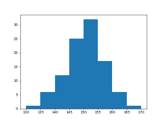
• 以下に統計処理の簡単な例題を示す

リスト : 統計処理の簡単な例 (sample03.py)

import numpy as np
import matplotlib.pyplot as plt

# 身長のデータ
height = [
    148.7, 149.5, 133.7, 157.9, 154.2, 147.8, 154.6, 159.1, 148.2, 153.1,
    138.2, 138.7, 143.5, 153.2, 150.2, 157.3, 145.1, 157.2, 152.3, 148.3,
    152.0, 146.0, 151.5, 139.4, 158.8, 147.6, 144.0, 145.8, 155.4, 155.5,
    153.6, 138.5, 147.1, 149.6, 160.9, 148.9, 157.5, 155.1, 138.9, 153.0,
    153.9, 150.9, 144.4, 160.3, 153.4, 163.0, 150.9, 153.3, 146.6, 153.3,
    152.3, 153.3, 142.8, 149.0, 149.4, 156.5, 141.7, 146.2, 151.0, 156.5,
    150.8, 141.0, 149.0, 163.2, 144.1, 147.1, 167.9, 155.3, 142.9, 148.7,
    164.8, 154.1, 150.4, 154.2, 161.4, 155.0, 146.8, 154.2, 152.7, 149.7,
    151.5, 154.5, 156.8, 150.3, 143.2, 149.5, 145.6, 140.4, 136.5, 146.9,
    158.9, 144.4, 148.1, 155.5, 152.4, 153.3, 142.3, 155.3, 153.1, 152.3
]

h = np.array(height)
print('sum = {}, max = {}, min = {}'.format(h.sum(), h.max(), h.min()))
print('mean = {}, var = {}, std = {}'.format(h.mean(), h.var(), h.std()))
print(np.histogram(h, bins=np.arange(130, 171, 5)))
print(plt.hist(h, bins=np.arange(130, 171, 5)))
# plt.savefig("hist.png", dpi=50)
plt.show()

$ python3 sample03.py
sum = 15062.699999999999, max = 167.9, min = 133.7
mean = 150.62699999999998, var = 41.389571000000025, std = 6.433472701426503
(array([ 1,  6, 12, 25, 32, 17,  6,  1]), array([130, 135, 140, 145, 150, 155, 160,
 165, 170]))
(array([ 1.,  6., 12., 25., 32., 17.,  6.,  1.]), 
 array([130., 135., 140., 145., 150., 155., 160., 165., 170.]),
 <BarContainer object of 8 artists>)

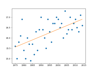
リスト : 東京の年平均気温 (sample04.py)

import numpy as np
import matplotlib.pyplot as plt

# 平均気温 (1975 - 2014)
data = np.array([
    15.6, 15.0, 15.8, 16.1, 16.9, 15.4, 15.0, 16.0, 15.7, 14.9,
    15.7, 15.2, 16.3, 15.4, 16.4, 17.0, 16.4, 16.0, 15.5, 16.9,
    16.3, 15.8, 16.7, 16.7, 17.0, 16.9, 16.5, 16.7, 16.0, 17.3,
    16.2, 16.4, 17.0, 16.4, 16.7, 16.9, 16.5, 16.3, 17.1, 16.6
])

x = np.arange(1975, 2015)

# 散布図
plt.plot(x, data, 'o')

# 相関係数
print(np.corrcoef(x, data))

# 回帰直線
a, b = np.polyfit(x, data, 1)
print(a, b)
plt.plot(x, x * a + b)

# plt.savefig('tokyo.png', dpi=50)
plt.show()

$ python3 sample04.py
[[1.         0.62750348]
 [0.62750348 1.        ]]
0.03442776735459678 -52.43618198874326

●乱数

• NumPy のモジュール random には乱数を生成する関数が多数用意されている
• rand(), [0.0, 1.0) の一様乱数を生成する
• randn(), 標準正規分布に従う乱数を生成する
• 引数に d0, d1, ..., dn を指定すると、乱数を格納した配列を返す
• randint(low[, high, size, dtype]), [low, high) の一様乱数 (整数) を生成する
• size は整数値またはタプル (shape)
• このほかにも、いろいろな分布の乱数を生成する関数が多数用意されている
• 詳細はリファレンスマニュアル Random sampling を参照

>>> np.random.rand()
0.047653528033401504
>>> np.random.rand(10)
array([0.7378687 , 0.24128895, 0.70803174, 0.70097538, 0.39710067,
       0.18238028, 0.7943424 , 0.12147911, 0.51665823, 0.68891523])
>>> np.random.randn()
-0.3073797959407569
>>> np.random.randn(10)
array([ 0.79187796,  0.00350009, -0.01247469, -0.59927661, -0.35585297,
        0.81813222, -0.09386419, -1.58999999, -1.43327989, -2.98426565])
>>> np.random.randint(0, 10)
7
>>> np.random.randint(0, 10, 20)
array([8, 9, 2, 5, 7, 9, 9, 9, 0, 1, 4, 4, 7, 2, 0, 4, 3, 9, 2, 9])
>>> np.random.randint(0, 10, (5, 5))
array([[0, 7, 7, 4, 3],
       [6, 0, 3, 1, 5],
       [6, 1, 0, 8, 4],
       [3, 2, 3, 9, 7],
       [7, 4, 1, 5, 9]])

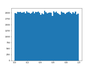
リスト : 一様分布 (sample05.py)

import numpy as np
import matplotlib.pyplot as plt

a = np.random.rand(100000)
plt.hist(a, bins=50)
# plt.savefig('rand.png', dpi=50)
plt.show()

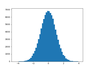
リスト : 正規分布 (sample06.py)

import numpy as np
import matplotlib.pyplot as plt

a = np.random.randn(100000)
plt.hist(a, bins=50)
# plt.savefig('randn.png', dpi=50)
plt.show()

リスト : モンテカルロ法で円周率を求める (sample07.py)

import numpy as np

n = 1000000
x, y = np.random.rand(2, n)
c = x ** 2 + y ** 2 <= 1
print(len(x[c]) / n * 4.0)

$ python3 sample07.py
3.141752

• メソッド choice() はランダムにシーケンスの要素を選択する
• 選択する要素の個数や、キーワード引数 p で確率を指定することができる
• shuffle() は配列をシャッフルする
• シード (種) の設定は関数 seed() で行う

>>> a = ['foo', 'bar', 'baz', 'oops']
>>> a
['foo', 'bar', 'baz', 'oops']
>>> np.random.choice(a)
'oops'
>>> np.random.choice(a)
'oops'
>>> np.random.choice(a)
'foo'
>>> np.random.choice(a, 2)
array(['bar', 'foo'], dtype='<U4')
>>> np.random.choice(a, 2)
array(['oops', 'foo'], dtype='<U4')
>>> np.random.choice(a, p=[1/2, 1/6, 1/6, 1/6])
'foo'
>>> np.random.choice(a, p=[1/2, 1/6, 1/6, 1/6])
'oops'
>>> np.random.choice(a, p=[1/2, 1/6, 1/6, 1/6])
'foo'
>>> np.random.choice(a, p=[1/2, 1/6, 1/6, 1/6])
'foo'
>>> np.random.choice(a, p=[1/2, 1/6, 1/6, 1/6])
'baz'

>>> b = np.arange(10)
>>> b
array([0, 1, 2, 3, 4, 5, 6, 7, 8, 9])
>>> np.random.shuffle(b)
>>> b
array([0, 2, 8, 5, 7, 1, 4, 6, 3, 9])
>>> np.random.shuffle(b)
>>> b
array([7, 8, 6, 1, 4, 9, 0, 3, 2, 5])

>>> np.random.seed(0)
>>> np.random.rand(10)
array([0.5488135 , 0.71518937, 0.60276338, 0.54488318, 0.4236548 ,
       0.64589411, 0.43758721, 0.891773  , 0.96366276, 0.38344152])
>>> np.random.seed(0)
>>> np.random.rand(10)
array([0.5488135 , 0.71518937, 0.60276338, 0.54488318, 0.4236548 ,
       0.64589411, 0.43758721, 0.891773  , 0.96366276, 0.38344152])